AI-Powered Phising Detection : How to unmask the outliers ?

This article is in English. Pour lire en français, consultez notre autres publications.

In today’s digital landscape, where cyber threats evolve at an unprecedented pace, traditional security measures often struggle to keep up. Cybercriminals continuously devise sophisticated tactics, leaving organizations vulnerable to breaches and data loss.

To combat these challenges, dynamic approaches to detecting cyber threats have emerged, leveraging the power of deep learning and machine learning.

Among these, outlier detection techniques stand out as a game-changing innovation. By identifying anomalies and irregular patterns, these methods allow security systems to pinpoint potential threats with greater accuracy and speed.

How to detect real threats ?

Deterministic approach with rule, the classic

The deterministic approach with rule-based systems is a cornerstone of traditional cybersecurity measures. This methodology operates on predefined rules and logic, where security policies and decisions are determined by a fixed set of conditions or signatures. For example, on specific IP addresses or ports based on these rules.

While this approach is reliable and predictable, providing clear accountability and ease of management, it often struggles against sophisticated, evolving threats. These challenges arise because deterministic systems rely on past knowledge of threats, leaving gaps in adaptability and proactive defense.

Despite its limitations, the rule-based deterministic model remains a foundational strategy.

Indeterministic approach with prediction

The indeterministic approach with prediction represents a modern shift in cybersecurity, leveraging probabilistic models and advanced technologies like machine learning and AI. Instead of relying solely on fixed rules or past threat patterns, this method predicts potential risks by analyzing vast amounts of data for anomalies, correlations, and behavioral patterns. For instance, predictive systems can detect unusual user behavior that may indicate a potential insider threat or uncover previously unseen attack vectors.

While this approach enhances flexibility and proactive defense, it also introduces challenges like managing false positives, the need for extensive computational resources and to have extensive datasets with equilibrated classification for training.

What is a lot of time missing.

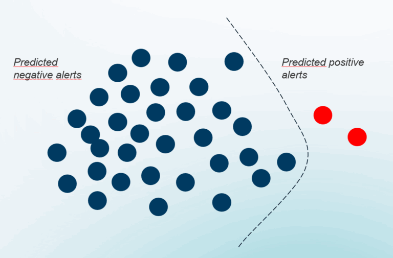
Indeterministic approach with outliers

The indeterministic approach with outliers focuses on identifying and analyzing anomalies that deviate significantly from normal behavior patterns (inliers).

For example, an unusually large file transfer or an atypical login location might flag as outliers, warranting further investigation. This approach is particularly effective at uncovering novel or hidden threats.

While powerful, it comes with challenges, such as distinguishing true threats from benign anomalies.

On the other hand, outlier detection does not require having a balanced dataset, just a healthy dataset with no threats inside.

The outliers approach

2 algorithms for maximum efficiency

Isolation Forest and Autoencoder are two distinct methods used for anomaly detection, each suited to different types of data and scenarios:

1. Isolation Forest is a tree-based method that identifies anomalies by isolating data points. This approach is particularly efficient with small datasets, as it has a low computational cost and does not require extensive training. It’s straightforward and performs well when data is compact and less complex.
2. Autoencoder, on the other hand, is a neural network-based method. It works by compressing the data into a reduced representation (encoding) and then reconstructing it (decoding). Anomalies are detected when the reconstruction error exceeds a threshold, as they deviate significantly from normal data patterns. Autoencoders are better suited for larger and more complex datasets, as they thrive on abundant data to learn intricate patterns effectively. They are highly flexible but can be computationally intensive and require proper tuning for optimal results.

In summary, Isolation Forest excels with smaller datasets due to its simplicity and efficiency, whereas Autoencoders shine with larger datasets, leveraging their ability to capture complex data structures.

How An Isolation Forest works

Isolation Forest works by constructing multiple decision trees to split data points based on random feature and value selections. The primary idea is that outliers, being rare and different, require fewer splits to isolate compared to normal points.

For example, an unusual data point far from the data cluster will quickly be separated, making it easy to identify as an anomaly. This efficiency in isolating outliers stems from their unique characteristics, which stand out in the dataset.

By aggregating the results from all the trees, the Isolation Forest method determines the anomaly score for each point, effectively identifying outliers in a robust and computationally efficient way

How Auto Encoder work ?

Autoencoders detect outliers by utilizing a latent space—a compressed representation of the input data—created during the encoding process. The encoder transforms the input into a lower-dimensional latent space, capturing essential patterns and features of the data while discarding less relevant information.

The decoder then reconstructs the data from this latent representation. Normal data points, which align with learned patterns, are reconstructed accurately, resulting in low reconstruction error.

Outliers, however, often fail to align with the structure captured in the latent space, leading to significant reconstruction errors. By analyzing these errors, the autoencoder identifies outliers as data points that deviate notably from the latent space’s learned patterns, making it an effective tool for anomaly detection in complex datasets.

It’s all about the treshold between inliers and outliers

In anomaly detection methods like Isolation Forest and Autoencoders, thresholds play a pivotal role in distinguishing inliers from outliers. For Isolation Forest, the anomaly score of each data point is calculated based on how easily it can be isolated within the dataset—outliers, being rare and distinct, are isolated faster. A threshold is then applied to classify points as either normal or anomalous.

Similarly, in Autoencoders, the threshold is based on reconstruction error. Data points that align well with the learned patterns in the latent space are reconstructed with minimal error, while outliers, which deviate significantly, exhibit higher reconstruction errors.

The threshold here determines whether a data point is flagged as an anomaly. In both systems, fine-tuning the threshold is critical to striking the right balance between catching true anomalies and avoiding false positives, making it the cornerstone of effective and reliable anomaly detection

Preparing the data : Normalization & enrichment

Example on phising data

To experiment with our outlier detection system, we focused on phishing scenarios using base logs from Microsoft Entra ID as our foundational dataset.

To enhance the data, we employed IPGeoLocation, enriching it with geographical context to better analyze patterns and anomalies.

For generating realistic phishing attempts, we utilized EvilGinx, a tool designed to simulate advanced phishing attacks.

This combination of enriched data and simulated threats allowed us to rigorously test the system’s ability to identify outliers, ensuring its effectiveness in detecting and mitigating phishing activities in real-world scenarios.

Our data pipeline

Our data pipeline begins with the raw input, consisting of diverse and unstructured data points. As the first step, we encode this data into binary format (0s and 1s) wherever possible, ensuring compatibility with analytical models.

Following this, we establish correlations by linking important contextual information, such as identifying whether a user is connecting from a new location or making a first-time access attempt.

After correlation, the data undergoes enrichment, incorporating additional threat intelligence, such as identifying malicious activities associated with IP addresses.

This enhancement adds valuable context to the data, enabling more informed anomaly detection.

Finally, the processed output is normalized and entirely composed of numerical values ranging from 0 to 1, ensuring streamlined and normalized integration into machine learning models for further analysis and decision-making.

Training the models

Library used

We utilized a range of powerful libraries to build and analyze our outlier detection system.

• PyTorch with CUDA was chosen for its ability to accelerate deep learning tasks by leveraging GPU capabilities, making it ideal for training Autoencoders efficiently on large datasets.
• Scikit-Learn provided versatile tools for machine learning and statistical modeling, particularly useful for implementing algorithms like Isolation Forest.
• NumPy was employed for its robust numerical computing capabilities, especially for handling arrays and performing mathematical operations.
• Pandas facilitated data preprocessing and manipulation, ensuring seamless handling of structured data.
• Seaborn and Matplotlib were used for visualisation, with Seaborn creating high-level statistical plots and Matplotlib allowing fine-grained control over visualizations.

Isolation Forest code example

# (Code Python Simplified)

import numpy as np
import random
from sklearn.ensemble import IsolationForest #Scikit-learn

rng = np.random.RandomState(42)

model= IsolationForest(n_estimators=300, max_samples="auto", contamination=0.005, random_state=rng, max_features=0.5)

def train(data):
   model.fit(data)

def score(row):
   return model.decision_function(row)

def predict(row):
   return model.predict(row)

Auto Encoder code example

# (Code Python Simplified)

import numpy as np
import torch
import torch.nn as nn
import torch.nn.functional as F

class AE(nn.Module):
    def __init__(self):
        super(AE, self).__init__()
        self.enc = nn.Sequential(
            nn.Linear(39, 16),
            nn.ReLU(),
            #nn.Dropout(0.1),
            nn.Linear(16, 8),
            nn.ReLU(),
            nn.Linear(8, 4),
            nn.ReLU(),
           
        )
        self.dec = nn.Sequential(
            nn.Linear(4, 8),
            nn.ReLU(),
            nn.Linear(8, 16),
            nn.ReLU(),
            #nn.Dropout(0.1),
            nn.Linear(16, 39),
            nn.ReLU(),
        )
    def forward(self, x):
        encode = self.enc(x)
        decode = self.dec(encode)
        return decode

model = AE()
device = 'cuda' if torch.cuda.is_available() else 'cpu'
model.to(device)
criterion = nn.MSELoss(reduction='mean')

batch_size = 32
lr = 1e-3         # learning rate
w_d = 1e-5        # weight decay
epochs = 60

optimizer = torch.optim.Adam(model.parameters(), lr=lr, weight_decay=w_d)

def train()
   # Use train_test loader
   for row in data:
      sample = model(row.to(device))
      loss = criterion(data, sample)
      optimizer.zero_grad()
      loss.backward()
      optimizer.step()

def score(row)
   with torch.no_grad()
      return model(row.to(device))

Results : is it working ?

Some numbers about performance & dataset

Our anomaly detection experiment utilized a dataset composed of approximately 6,000 True Negative items and 8 True Positive items.

For training, we randomly sampled 5,400 True Negative instances, while the test dataset consisted of 600 True Negative samples and 8 True Positive items.

Regarding performance, the Autoencoder demonstrated impressive efficiency with 28 seconds of training, distributed over 30 epochs, each taking 960 milliseconds. Inference was remarkably fast, averaging just 2.4 milliseconds, thanks to the powerful 3080 GTX GPU (Graphical card) with 8,074 CUDA cores.

On the other hand, the Isolation Forest showcased its speed with only 840 milliseconds of training and 25 milliseconds for inference, optimized by a robust i9 CPU (Processor) featuring 24 cores and 64 GB of RAM.

These results highlight the Autoencoder’s suitability for large-scale deep learning with a GPU, while Isolation Forest provides rapid deployment for only CPU calculation.

PCA (Principal component analysis)

What is PCA ?

Principal Component Analysis (PCA) is a statistical technique commonly used in data preprocessing and dimensionality reduction. It works by identifying the principal components—essentially the directions in which data varies the most—and projecting the data onto these components.

PCA transforms the original high-dimensional dataset into a lower-dimensional representation, capturing the most significant patterns while discarding less relevant noise or variance. This method is particularly useful for simplifying complex datasets, enhancing visualization, and improving the efficiency of machine learning models.

Here we reduce 39 dimensions into 2 for visualize it.

Analysis of the charts

The phishing attempts are clearly clustered in a consistent region within the data, demonstrating the effectiveness of our enrichment and normalization processes.

By refining the raw data, we successfully enhanced the quality and uniformity of the dataset, making it easier for anomaly detection systems to operate efficiently.

When comparing the performance of the two models, the Auto Encoder showed slightly better results.

However, the Isolation Forest also performed commendably.

Overall, both approaches demonstrated strong capabilities in identifying phishing attempts, validating the robustness of the data preparation and the models themselves.

Anomaly score distribution

When analyzing the anomaly score distribution charts, distinct patterns emerge for the Autoencoder and Isolation Forest models.

On the Autoencoder chart, there’s a striking explosion of frequency concentrated on the left side, represented by a massive bar, while the right side remains notably empty. This sharp distribution indicates that the Autoencoder effectively segregates normal data points from anomalies. The vertical green lines marking phishing attempts clearly fall after the red dotted threshold line, demonstrating that the model successfully detected all phishing anomalies with a high reconstruction error.

In contrast, the Isolation Forest chart shows a more even distribution of anomaly scores, with no dramatic spikes. While most phishing attempts are correctly identified, some fall to the left of the red dotted threshold line, indicating that they were undetected.

This smoother distribution reflects the probabilistic nature of Isolation Forest and its broader approach to isolating outliers. While effective overall, it leaves room for improvement in capturing subtle anomalies like phishing attempts compared to the Autoencoder.

Both models demonstrate strengths, but their unique distribution patterns highlight differences in their detection capabilities

Precision – Recall

What is Precision – Recall ?

Precision and recall are two metrics used to evaluate the performance of classification models, particularly in detecting anomalies or specific categories.

Precision measures the proportion of correctly identified positive cases (true positives) out of all predicted positive cases, highlighting how accurate the model is when it claims something is positive.

Recall, on the other hand, measures the proportion of true positive cases that were correctly identified out of all actual positive cases, indicating the model’s ability to detect positives without missing any.

For example, imagine a spam email detection system: if it flags 10 emails as spam and 8 of them are truly spam (precision = 80%), but there are 20 spam emails in total, and the system only identifies those 8 (recall = 40%), the model is highly precise but lacks recall.

Balancing precision and recall is crucial for optimal performance, depending on the application’s priorities.

Analysis of the charts

On the precision-recall chart of the Autoencoder, we observe that precision remains consistently strong but gradually decreases as recall grows.

This behavior highlights a trade-off, as increasing recall captures more potential threats but slightly reduces precision.

Notably, the best point is at recall of 1, where all true threats are correctly identified.

In cybersecurity, this is crucial because discarding even a single true threat can have severe consequences, making this high-recall approach highly valuable.

In contrast, the precision-recall chart for Isolation Forest appears more spiky, with precision fluctuating alongside recall.

The optimal point is observed at recall of 0.8 and precision of 0.8, reflecting a balance where most true threats are detected without excessive false positives.

F1 Score

What is F1 Score ?

The F1 score is a metric that combines precision and recall into a single value to evaluate the balance between these two measures. It is the harmonic mean of precision and recall, calculated as:

F1 = 2 × (Precision × Recall) / (Precision + Recall)

For example, consider a phishing detection system: if the system flags 10 phishing attempts, and 7 are correct (precision = 70%), but there are 14 actual phishing attempts in total, and the system only identifies 7 of them (recall = 50%), the F1 score would be 58%.

The F1 score is particularly useful when there’s a need to balance both precision and recall, such as in cybersecurity, where detecting all threats is vital while keeping false positives manageable.

Analysis of the charts

On the F1 score chart for the Autoencoder, we observe an impressive peak at 0.96, reflecting a near-perfect balance between precision and recall. This exceptional score highlights the Autoencoder’s capability to effectively identify phishing attempts while minimizing false positives, making it highly reliable.

On the F1 score chart for the Isolation Forest, the maximum score drops slightly to 0.86. While this is lower compared to the Autoencoder, it still indicates a strong performance, demonstrating the Isolation Forest’s ability to detect outliers with reasonable accuracy and efficiency.

Confusion matrix

What is a Confusion Matrix ?

A confusion matrix is a table used to evaluate the performance of a classification model by comparing its predictions to the actual outcomes.

It consists of four key values: True Positives (TP), where the model correctly predicts the positive class; True Negatives (TN), where it correctly predicts the negative class; False Positives (FP), where it incorrectly predicts the positive class; and False Negatives (FN), where it misses the positive class.

For example, imagine a spam detection system: if there are 10 emails, 6 of which are spam and 4 are not, the model might correctly classify 5 spam emails (True Positive TP) and 3 non-spam emails (True Negative TN), but it mistakenly marks 1 non-spam email as spam (False Positive FP) and misses 1 spam email (False Negative FN).

The confusion matrix summarizes these results, offering a clear picture of the model’s accuracy and error rates in another ways than Precision-Recall chart.

Analysis of the charts

The confusion matrix for the Autoencoder reveals a highly effective performance, with no False Negatives. This indicates that the model successfully detected all phishing attempts, ensuring that no genuine threats were overlooked—a critical aspect in cybersecurity.

However, it did show a small number of False Positives, suggesting that the model is slightly over-sensitive, flagging some benign cases as threats.

On the other hand, the confusion matrix for the Isolation Forest highlights a less robust performance, with some False Negatives where phishing attempts went undetected.

Additionally, it also showed False Positives, emphasizing a lower overall reliability compared to the Autoencoder.

These results demonstrate that while both models are effective, the Autoencoder outperforms the Isolation Forest in accurately identifying phishing attempts and minimizing overlooked threats.

Do we have overfitting ?

What is Overfitting ?

Overfitting occurs when a machine learning model becomes too specialized in recognizing patterns within the training data, including noise or irrelevant details, rather than generalizing to unseen data. This leads to high accuracy on the training data but poor performance on test or real-world data.

For example if the model focuses excessively on unique features of the training phishing samples—like specific IP addresses or email templates—it may flag these perfectly during training. However, it might fail to identify new phishing attempts that don’t match those exact details, as it hasn’t learned broader, generalizable patterns.

Analysis of the charts

In the overfitting detection chart for anomaly score distribution using Autoencoders, we can see a comparison between the train and test datasets that reveals no significant peak differences. The anomaly score distribution follows a smooth, descending linear slope across both datasets, indicating minimal overfitting.

On the Isolation Forest overfitting detection chart, the anomaly score distribution shows a different behavior. While there are more peaks and variations caused by less pronounced clustering, the results for the test dataset remain relatively linear.

This linearity demonstrates that the Isolation Forest is also successful at generalizing the learned patterns, despite having more fluctuation in scores.

Challenging the results

The results of our anomaly detection experiment on phishing events reveal solid performance from both models, though they are not without room for improvement.

The precision, recall, and F1 scores are strong, with the Autoencoder achieving an impressive F1 score of 0.96 (excellent), while the Isolation Forest reaches a respectable 0.86 (good).

As expected, the Autoencoder, a neural network-based model, outperforms the Isolation Forest, a decision-tree-based model, especially given the dataset size.

With a small dataset of 6,000 items, the Autoencoder requires a minimum of 5,000 data points for effective training, while the Isolation Forest can perform well with as few as 300.

The synthetic true positives phishing attempts created with EvilGinx prove that the dataset could certainly be further enriched for more realistic results, however, with the typical caveats that come along with synthetic data.

Moreover, enhancing the input through feature engineering, adding more data correlation, tuning hyperparameters, and experimenting with different dataset sizes could further boost model performance.

Why Auto Encoder model have better result on Isolation Forest model ?

The Auto Encoder model achieves better results than the Isolation Forest model primarily due to its ability to learn complex patterns and representations within the data.

As a neural network, the Auto Encoder compresses data into a latent space, capturing intricate relationships and subtle variations that might be missed by simpler models. This is particularly advantageous in scenarios with high-dimensional or complex datasets, as the Auto Encoder can adapt to nonlinear patterns.

In contrast, the Isolation Forest relies on a decision tree-based approach, which isolates data points based on randomness and tends to be less effective in capturing nuanced patterns.

Furthermore, the Auto Encoder benefits from leveraging extensive training epochs, allowing it to refine its understanding of anomalies more thoroughly.

While Isolation Forest is faster and efficient with small datasets, its simpler structure limits its ability to match the nuanced detection capability of Auto Encoders, leading to comparatively lower output performance but still with better compute performance.

What’s next ?

Our experiments have validated the effectiveness of both Auto Encoder and Isolation Forest as strong algorithms for detecting phishing threats.

The Auto Encoder demonstrated superior precision, recall, and F1 scores, making it particularly adept at capturing complex patterns in the data.

However, the Isolation Forest also showed commendable results, proving itself as a reliable and efficient alternative, especially for smaller datasets.

These findings establish a solid foundation for anomaly detection in phishing but for others threats domains too.

The next step is to advance this work by incorporating more realistic and diverse datasets, moving beyond synthetic data to reflect real-world scenarios.

Deploying these models into a production environment will not only challenge their robustness but also push the boundaries of this indeterministic approach, driving innovation and refining their ability to detect and mitigate phishing attempts at scale.